1.2. GNSS Component Products

The GNSS product consists of a set of displacement time series, one for each station within the region of the CGM—nominally defined as 123.0°W–113.5°W longitude, 30.0°N–38.0°N latitude—and a velocity solution. Time series files are provided in the GAGE’s comprehensive “.pos” format and a script allows simple conversion to one of many other common formats, e.g. the Nevada Geodetic Laboratory’s (NGL’s) .txyz2 and .tenv3 formats, a free-format GeoCSV (e.g. http://geows.ds.iris.edu/documents/GeoCSV.pdf) and GMT’s “psxy” format. (Eventually, the GeoCSV format may be made the primary CGM format due to its potential for arbitrary expansion and the conversion script will be completed for all possibilities.)

Each time series file contains metadata in the header related to the station’s identification, nominal location and length of time series. Data from both survey (campaign) and continuous GNSS stations are provided, from mid-1991 to the present for the survey stations and from 1994 for the continuous stations. The survey time series are provided by Zheng-Kang Shen (UCLA) and colleagues, and the continuous time series are combined by Mike Floyd (MIT) and colleagues from several source analysis centers [Figure 1.1]. The continuous time series are updated weekly with new data from the ingested analysis centers.

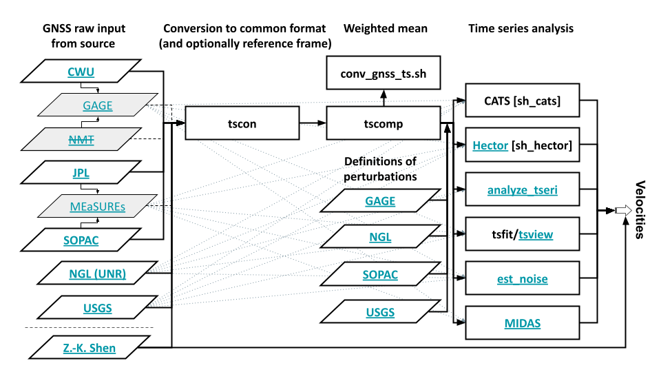
Figure 1.1 The workflow of the SCEC CGM GNSS product, showing source analysis centers (left column; white outlined in bold), correction and combination programs (middle), and algorithms contributing to the analysis of the resulting consensus time series (right).

The GAGE (CWU), JPL, NGL (UNR) and USGS time series products are all processed using the Gipsy software, and the SOPAC time series are processed using the GAMIT/GLOBK software. Previous studies and analyses have shown that final reference frame transformations applied to the Gipsy time series include a scale term that can suppress signals in the local vertical component potentially related to geophysical phenomena rather than reference frame artifacts [Herring, 2015, Herring et al., 2016]. We therefore restore the scale estimate provided in JPL’s “x”-files. (In the case of the current USGS products, a previous set of “x”-files are used up to and including 2018-05-26; J. Svarc, pers. comm.) It is also readily evident that the sigmas associated with data points in time series processed with Gipsy are much smaller than those processed with GAMIT/GLOBK [Herring et al., 2016], likely due to a difference in the approach to weighting raw phase data at low versus high elevations, where perturbing atmospheric noise is larger and smaller, respectively. So we rescale sigmas for all stations and all components by a constant value per input Gipsy-based analysis center, which produces a normalized root-mean-square residual of ~ 1 at stations that are used to redefine a consistent reference frame before final combination [Table 1.1]. Each analysis center’s time series are already aligned to a given terrestrial reference frame but we also realign each set of time series, for consistency before averaging, using the same set of stations to define four different reference frames: IGb14, the second IGS realization of the ITRF2014 no-net-rotation reference frame cite:p:Altamimi_et_al_2016; North America and the Pacific, defined by the ITRF2014 Plate Motion Model [Altamimi et al., 2017]; and North America defined by Kreemer et al. [2018]. Finally, the consensus CGM time series are generated by simple weighted averaging [Equation (1.1)], where the associated uncertainty for each point is the inverse of the square root of the sum of the weights (inverse variances) for each station i, rescaled by the square root of the total number of contributing solutions, n [Equation (1.2)]:

(1.1)\[\bar{x}_i\left(t\right) = \frac{\sum_{i=1}^n x_i\left(t\right)/\sigma_i^2\left(t\right)}{\sum_{i=1}^n 1/\sigma_i^2\left(t\right)}\]

(1.2)\[\bar{\sigma}_i\left(t\right) = \frac{\sqrt{n}}{\sqrt{\sum_{i=1}^n 1/\sigma_i^2\left(t\right)}}\]

Table 1.1 Sigma rescaling constants applied to time series from analysis centers processing with Gipsy. The constant is used to multiply the time series sigmas for all components at all stations.

Analysis center	JPL	NGL (UNR)	USGS
Sigma multiplication factor	2.3	2.2	2.1