GAMIT/GLOBK MATLAB TOOLS
Thomas Herring and Simon McClusky, MIT
Last Updated 4/4/09 8:16 AM
Comments should be sent to tah@mit.edu
This software is covered by the standard GAMIT/GLOBK License agreement.
Content
|
Vers |
Introduction to the tool box |
|
|
|
Instructions for installing and running programs either in Matlab Ver 7 or stand-alone programs |
|
|
|
History of changes to the programs |
|
|
2.01 |
Velocity field viewing tool including profiling and interface to tsview |
|
|
2.02 |
Time series viewing, editing and interface to GLOBK |
|
|
|
|
|
|
GAMIT/GLOBK
MATLAB TOOLS Content Running as standalone programs Ensum file: Not implemented
in Ver 1.0 Example screen view and output |
Overview
These tools are provided as a means to help users understand the quality of the results being obtained from GLOBK analyses of GPS data. Their primary aim is to improve the quality and understanding of the results from large GPS analysis projects.
Installation
The latest tsview/velview mfiles are saved in GGMatlab_mfiles.tar. When running from MATLAB this verion of the m-files should be downloaded. The m-files are in a folder called matlab and in this folder are folders for tsview and velview.
To run the velview and tsview programs you should download the Matlab® mfiles for either x86_64 (GGMatlab_x86_64.tar) or for Intel Mac OSX (GGMatlab_maci.tar). These tar files are identical except that each tar file contains the executable program for their respective systems (see details below). The tar files contain directories for velview and tsview. If you have a license for Matlab you can go to the section Running under Matlab® after the files have been untarred.
If you do not have a license for Matlab, you should download MCRInstaller.bin for x86_64 systems or MCRInstaller.dmg for Intel Max OSX (These files are each 300Mbytes). Once the appropriate file is downloaded, follow the instructions in the Running as standalone programs section after the tar files above have been untarred.
The tar files contain directories for tsview and velview. The executaubles are in these directories along with the Matlab m-files. The tar files can be untarred in any convenient directory. For GAMIT/GLOBK users, the untarred directory can be put at the level of gamit, kf, and library directories. Also available is an example case saved as Example.tar. The examples below use the data in the Example directory. This directory can be placed anywhere in your system.
Instructions: In the directory where you plan installing the software, you should untar the tar file for the system you are using..
% tar xvf <Download_Directory>/GGMatlab_x86_64.tar
or
% tar xvf <Download_Directory>/GGMatlab_maci.tar
where < Download_Directory> is the directory where the GGMatlab tar file is located
Below we refer to the x86_64 or maci directories as <matlab_dir>
Running under Matlab®
To run with Matlab Release 2006a or later.
Either add the paths to your startup.m in the matlab directory of your home directory by adding:
addpath <matlab_dir>/velview
addpath <matlab_dir>/tsview
or at the Matlab prompt after starting matlab, type the above two lines (the former approach is the preferred method).
>> velview
or
>> tsview
at the Matlab prompt will start the programs (See notes below on being in the correct directory when starting tsview.)
NOTE: On Mac OSX for matlab versions prior to release 2009a, the input boxes in both velview and tsview are much more readable if matlab is started as matlab –nojvm
This is a quick start to matlab that does not invoke the
Java Virtual Machine (JVM). The
executables are generated this way.
The nojvm option may be used R2009a but will generate a warning message
each time a new figure is created.
Running as standalone programs
The current distribution includes executables for Linux 32-bit (gcc 4.0 and greater) and Intel Mac OSX (10.5).
Two steps need to be taken to run the executable versions of velview and tsview.
(1) Install the matlab libraries by either running
MCRInstaller.bin on linux or my mounting MCRInstaller.dmg and then installing
on Intel Mac OSX. Follow the
instructions given by the Installers and note where the matlab libraries are
installed. On linux there is no
specific location for these to be installed. On Mac OSX, the default will be /Applications/MATLAB/MATLAB_Compiler_Runtime/v78. We will refer to this directory are
<mcr_root>. The instructions
below are also included in the readme.txt files in the tsview and velview
directories.
(2) Environment setup. This setup differs between Linux and OSX. CAUTION: Some browsers may add line breaks to the long setup lines below and so we have also included this information in Setup.txt.
For Linux: In your .cshrc file (bash users should set the corresponding path and export variables).
# (a) Add path information
set ggm = <matlab_dir> # <matlab_dir is the name of directory where x86_64
directory was installed.
set ggmpath = (${ggm}/tsview ${ggm}/velview )
set path = ($path $ggmpath)
# (b) Add library information
set mcr_root = <mcr_root> # <mcr_root> is the
directory where Matlab libraries were installed
set MATL_LIB =
${mcr_root}/bin/glnxa64:${mcr_root}/sys/os/glnxa64:${mcr_root}/runtime/glnxa64
setenv XAPPLRESDIR ${mcr_root}/X11/app-defaults
setenv LD_LIBRARY_PATH <Any existing LD_LIBRARY_PATH>:${MATL_LIB}
# Needed for 2008a Matlab exectuables
alias tsview `which tsview`
alias velview `which velview`
For Intel Mac OSX
# (a) Add path information
set ggm = <matlab_dir> # <matlab_dir is that name of directory where tsview/velview
directory was installed.
set ggmpath = (${ggm}/tsview ${ggm}/velview )
set path = ($path $ggmpath)
# (b) Add library information
set mcr_root = <mcr_root> # <mcr_root> is directory
where Matlab libraries were installed
/Applications/MATLAB/MATLAB_Compiler_Runtime/v78 by default
setenv DYLD_LIBRARY_PATH ${mcr_root}/runtime/maci:${mcr_root}/sys/os/maci:${mcr_root}/bin/maci:/System/Library/Frameworks/JavaVM.framework/JavaVM:/System/Library/Frameworks/JavaVM.f
ramework/Libraries
setenv XAPPLRESDIR ${mcr_root}/X11/app-defaults
Because of wrapping problems in the text, we have put a
version of the above lines in Setup.txt which can be
pasted into ~/.cshrc after the directories names have been updated with the
appropriate values.
There is also a readme.txt in the tsview and velview directories that explains these steps. There is no need to use the run_tsview.sh or run_velview.sh scripts. (Although these can be used to test if the deployedMCRroot is correct).
Modifications
Velview
From Version 1.00
- Fixed problem with display of number of sites in the secondary field during pan
- Fixed TeX error when site name includes _ in the first four characters.
- Fixed non-removal of vertical error bars on re-draws.
- Fixed small problem with variance calculation in CloseStats code.
- Clarified some of the documentation.
- Added Align button to remove offset from secondary field
From Version 1.01
- Added mb_ file directory specification in velview
- Added ID button
- Added features option to plot coastlines, faults and earthquake locations. (Feature does not work in executable, file not found message)
From Version 1.01
- Fixed some small problems with zero sigma velocities (sigma replaced with 0.1 mm/yr) and velocities that have no range when plotting profiles.
From Version 1.02 to 2.00
- Added
capability to read PBO formatted velocity fields.
- Added
Print dialog box for the executable version to control printing.
From Version 2.00 to 2.01
- Changed color scheme and plotting of vertical motions so that positive and negative velocities appear with different colorsvel
Tsview
From Version 1.00
- Added specification of directory for mb_ files
- Added Logarithmic fit and the ability to textually edit break types
From Version 1.01
- Added “Realistic Sigmas” calculation that using changes in chi-squared with different averaging intervals to extrapolate to a long-term velocity sigma.
- Added Averaging of time series residuals.
From Version 1.02 to 2.00
- Fixed problems with Version 7 Matlab compatibility problems
- Updated to read PBO formatted time series position files
- Added button to allow removing of error bars.
From Version 2.00 to 2.01
- Added ability to read GLOBK earthquake files
From Version 2.01 to 2.02
- Added additional buttons that control whether coseismic displacements are removed when linear-only residuals are plotted, and specify if time series of log corrects are output as PVO files.
- Allowed names with different frames so search for .pos file
Velview
Aim: The primary aim of velview is to view and assess the quality the velocity fields generated by GLOBK. The files read by velview are either standard globk velocity files (extracted with sh_exglk –f <input globk org file> -vel <output velocity file>) or PBO velocity files (See http://pboweb.unavco.org/dmsdocs/Root%20Folder/Data%20Management/Data%20Product%20Documentation/gps_velocity_format.pdf )
Typing velview at the Matlab prompt or from a terminal window generates the new figure shown below. All the buttons have tips shown when the cursor is passed over them.
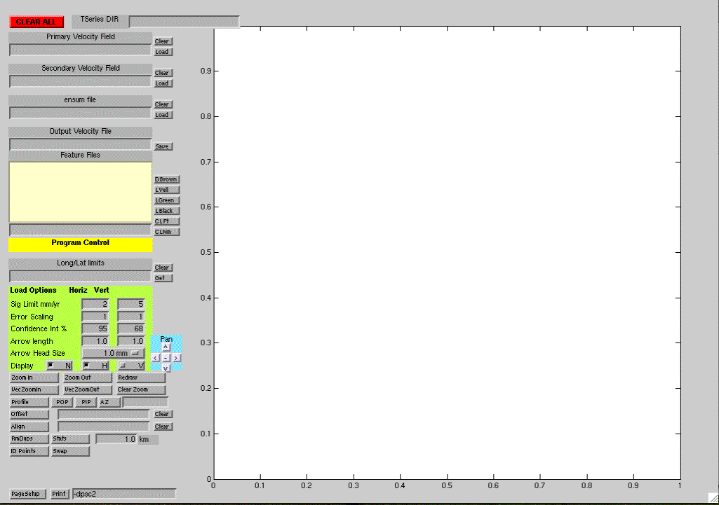
Basic uses of velview.
General comments
Velview allows many levels of interactions with the displaying velocity fields and multiple changes to the display can be made at one time. As a general rule, if multiple changes are made at the same time, use the redraw button to ensure that the figure is rendered correctly.
The current version of velview has problems crossing the zero longitude line, i.e., longitudes near 360 degrees are not converted to negative values. If needed the CLEAR ALL button should remove most of the plot, allowing it then to be re-constructed.
If very large velocity vectors are present, it is sometimes necessary to set the "arrow length" entry to a small value for the file to be read
Primary Velocity Field
The first action when velview is started is to type the name of a GLOBK velocity field file in the Primary Velocity Field box and then click the Load button next to it. (Hitting return in the text box will NOT load the field. Use of the Load button is required). This action will read the velocity field information from the file named and plot the velocities with the default conditions. (Since the figure is auto-scaled to fit with velocity vectors shown at “real” scale (i.e., 10 mm/yr will be 10 mm on the computer screen), you should be careful that there are not excessively large values in the velocity estimates).
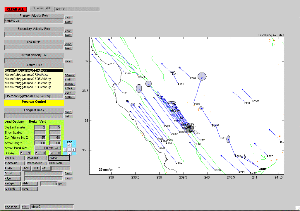
In the Examples directory, using the ParkEX.vel file will generate the following plot. (The Features option and Time Series DIR has also been used on this plot)
Time Series DIR
The directory name in this box will be used to find the times series files for plotting with tsview when a velocity vector is selected and the time series requested.
Secondary Velocity Field
The Name of a secondary velocity field can be specified in the text box and the Load button clicked. The geographic scales (ie., lat and long ranges) are retained from the current view when the secondary field is loaded. If there are no numeric values in the Lat/Long limits box, the geographic scales are reset when the primary field is loaded.
Ensum file: Not implemented
Output Velocity File:
The name is entered in the box and Save pressed. Entries in the primary and secondary fields are written to the output but duplicates in the secondary file are written as comments.
Feature Files
Included in the GAMIT/GLOBK maps directory are several Matlab readable files that contain the California Coast (CCVelV.xy), major faults (CF3VelV.xy), and earthquake locations of magnitudes >2, >3 and >4 since 1996. These can be plotted on the figure and will remain there until the CLEAR ALL button is pressed. Subsequent figures have these features plotted (cc shown with black line (LBlack) and faults shown with green lines (LGreen), and earthquakes with brown dots (DBrown). Feature files can be selected and the line/dot style changed or cleared. The CLNm (clear name) button can be used to clear the name from the text box. When changing the way a feature is drawn, the name box should be empty. The CLFt button will remove the selected feature form the plot (again name box must be empty).
Long/Lat limits
If this box is left blank then the limits are automatically calculated to show all sites and their velocity vectors. (There can be problems with the algorithm used for very large velocity vectors. Setting the arrow length to a small value can be used to read these files). The Get button will copy the limits on the current plot to the box and future Loads will display with these limits. The Clear button a convenient way of erasing the values in the box. The Long/Lat limits only affect loading of data.
The Load Options
The first two load options have effects only when data is loaded (Sig Limit and Error Scaling). The other options can be changed and bought into effect by clicking the Redraw button.
Sig Limit : Limits on the velocity uncertainties when the data are loaded. If the V box (see below is set), then both the horizontal and vertical velocities must satisfy the conditions. The limits are checked before Error Scaling.
Error Scaling:
Multiplier on the sigmas in the data file. Both the Sig Limit and Error Scaling may be changed between
loads of the primary and secondary fields.
Confidence Int: Changes the confidence intervals for the error ellipses and vertical velocity error bars. May be updated with the Redraw button.
Arrow Length: Scaling between the plotted lengths of vectors and height velocities and approximately real size on the computer screen (depends on monitor size).
Arrow Head Size: Sets the size of the arrow heads in millimeters relative to millimeters of vector length (e.g, with 1 mm arrow heads, a 1 mm/yr velocity would be the same length as the arrow head. Redraw causes the update.
Display: Sets the contents of the figure: If checked then, N selects site names, H selects horizontal velocities and V selects vertical velocities. Redraw causes the update.
Pan buttons:
These four buttons pan the view by half the width or height depending the button pressed (e.g., ^ shows sites at higher latitudes). The fifth button in the center zooms the figure out by 50% while retaining the vector lengths.
Zoom buttons.
Velview uses two types of zooms. The Zoom In and Zoom out buttons act like the normal Matlab zoom in that the vectors will increase in size with zoom in. (The Arrow length box updates to show the new length of the arrows). After the first Zoom in, the Zoom out button turns green and clicking it will reverse the sequence of Zoom Ins.
Vec Zoomin and Vec Zoom Out preserve the vector length on zooms. Again the Vec Zoom Out button turns green when it can be used and reverses the sequence of Vec ZoomIn. Strange arrow lengths can result if the Zoom Out buttons are used in an order different to the Zoom in sequence. A new arrow length can be typed in the Arrow Length Box and Redraw will bring the vectors back to a known length. (The arrow length box should give the actual value being used but it might be a strange value.)
For both zoom in buttons, the sequence is to click the Zoom In or Vec Zoom In button, and then in the figure window, click and drag (i.e., move while keeping the mouse button pressed) the area to be viewed in detailed. This sequence can be repeated as many times as needed. The Zoom Out buttons then reverses the sequences. Note: An area larger than the figure can be selected and the Zoom In then acts like a Zoom Out.
Redraw button
Clicking this button redraws the plots with the current settings in the Load Options. After multiple changes in the settings of the figure, this button should always be used to ensure that the figure is rendered correctly.
Profile Buttons
The Profile line of buttons control setting up profiles to be displayed and evaluated. By default, velocity vectors will be projected into a direction along the profile and at 90 degrees (counter clockwise) to the profile. However the azimuth for the projection can be set in one of two ways: (a) A value can be typed into the box to the right of the Az button or (b) the Az button can be clicked which allows graphical input. After the Az button is pressed, click in the figure window and drag the direction you want the vector projected onto. When the mouse button is released a dark blue line will appear for a second showing the azimuth selected and the value will be written into the Az box.
The velocities shown in the profiles are only from the primary field and do not have the offsets removed that may be applied to the velocities (see Offset below)
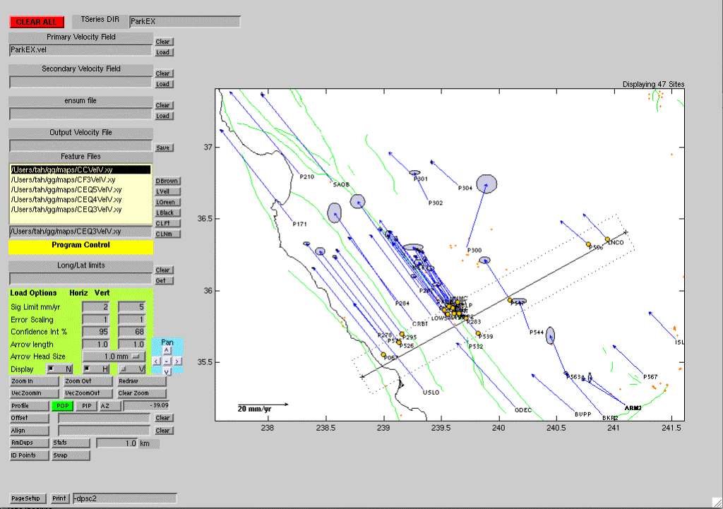
To select the profile: click the Profile button and then move to the figure window. Click where you would like the profile to start and drag out the centerline of the profile. When the centerline is in the correct location, release the mouse button and click again. Drag away from the centerline to make a box that will expand to show the area to be included in the profile. When the mouse button is released the second time, sites in the profile will be marked by yellow circles; the characteristics and list of sites in the profile box will be written to the Matlab window (or terminal screen); and a Profile Figure will pop-up.
The velview selection and the profile figure are shown below.
Profile Figure:
The figure below has a number of the features of the profile module already used.
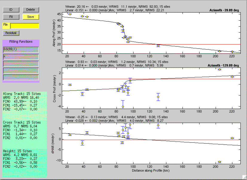
The main features of the Profile Figure are:
ID: Allows points to be identified (information appears on the left hand side of the figure. By using right-button-click, multiple points can be identified.
Delete: Allows points to be deleted. An X is over printed on the point to show that it has been deleted and a message (in red) appears at the bottom-left corner of the window.
Fit: Allows functions to be fitted to the profile. The functions to be fitted are typed in the Fitting Functions boxes when velview is run from within Matlab. When velview is run as an executable, only the SS and x function, as shown above, can be used. The x function is just a linear function. The SS function is a Okada model for a strike slip fault and is the equivalent to
SS(D,H) = 1/2+atan((x-D)/H)/pi,
where x is the distance along the profile, D is the distance to the fault and H is depth of the locked portion of the fault. In the example above we have chosen D to be 89 km and the locking depth 1 km (this is profile is in the creeping section of the San Andreas fault).
The estimates appear on the left side of the screen for the Azimuth directions shown on the plots. The WRMS is in mm, and the NRMS is the square root of chi squared per degree of freedom. FCN0 is always an offset, and FCN1-5 are the parameters of the functions typed in. The estimates text may be removed by clicking them. (Multiple estimates will stack in the same location on the plot.)
File and Save buttons allow the information about the profile to be saved. The lines in these files start with certain strings so that the file can be grep’d (to generate input to GMT for example). The output of the above profile can be found here. (ParkEX_prof.dat)
Residual button will plot the residuals to the profile fit. (To replot the original profile, select the Fit button).
Other Profile buttons:
POP and PIP button remove the profile boxes from the main velocity field figure. POP removes the last one plotted, while PIP removes the initial one plotted. The POP stays green while ever there are profiles still plotted on the figure.
Offset row
Clicking the Offset button will remove offsets from the primary and secondary velocity fields (same offset for both fields). If there are numerical values in the box next to the Offset button, these will be applied to the field (for example after a field is loaded). If the original velocity fields are in different frames the GLOBK utility program velrot can be used to align them before viewing in velview. If the box is empty, either by erasing its contents or by using the clear button), a click and drag box is used to select a square region from which the weighted-average value will be computed. A text window appears on the figure showing the statistics of the fit plus these results are written to the Matlab window. Clicking the text box will remove it from the screen.
Alignment row
The align button computes offsets between the secondary and primary velocity fields as simple additions to the North, East and Up velocities. For small areas, these offsets will account for frame differences between the two fields. For larger areas, the velrot program should be used before hand to bring the fields into alignment. If the box next to the button is empty, a click-drag technique us used to select the area in which the alignment parameters are computed. If the site names match the secondary and primary fields, these sites are used to compute the alignment. For sites in the area that do not have matching site names, sites within the separation distance are used. If the site separation is set to zero then only sites with the same names will be used in the alignment. The output written to the figure window can be removed with a click in the window.
RmDups and Stats
The RmDups button is used to remove duplicate site names that are within specified separation and that have the same velocity. (Results from using the equate option in GLORG). The duplicate sites are removed and will not appear in output files.
The Stats button computes the statistics of the differences in velocity for nearby sites (within the separation distance) and writes the results to the Matlab window. Only the sites in current view are used to compute the statistics of the differences. A file, Diff.vel, is automatically created with differences given in a velocity field format.
ID Points
Allows the identification of points inside a “click and drag” box on the velocity plot. The screen output may be removed by clicking on it.
SWAP
Allows the primary and secondary velocity fields to be swapped. This is useful when making profiles since only the primary field velocities are shown on the profile plots.
Print and Page Setup:
These buttons allow the page setup (paper orientation, fitting of the figure on the page) to be set. The print button prints the figure using the arguments given in the box next to it. Some typical options are:
-d<device> with device being psc for color post script; png for portable network graphics; jpeg forjpeg image
-r<NN> sets resolution for image formats. NN is dots per inch with 72 being appropriate from screen resolution.
-P<queue> to set the printer queue to be used
<filename> the last argument can be a file name to which the print is sent.
Example: -djpeg –r72 Test.jpg outputs figures to jpeg file.
The -noui option needs be used in the executable version. This option removes the GUI controls from the printed output.
When run under Matlab, the functionality of these boxes is available under the file menu.
In Figure Actions
The velocity vectors plotted by velview are active in that clicking on a vector brings up a menu box that can be used to get information about the velocity vectors.
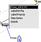
The menu items here each have an action. The top line shows the site name and the field it is from F1 is the primary, F2 is the secondary. Clicking on the site name will make the box disappear and no other actions will take place.
LabelOnFig will write information about the site position and velocity on the figure near the site name. Clicking on this label will make it disappear.
LabelPopUp will write the same information but on a new window that will appear in the upper right corner of the computer screen. This window may be destroyed using the normal close window techniques.
TimeSeries will launch tsview for this station (see Tsview section). The time series files will be searched in the Time Series DIR location. If this field is blank then the current directory will be used.
Delete will delete the site from the velocity field and the figure. There is no undo feature. If a site is accidentally deleted, the field will need to be re-Loaded.
![]()
Tsview
Aim: The primary aim of tsview is to assess the quality of time series generated by GLRED runs and to generate control files for GLOBK that will delete bad site position estimates and account for jumps in time series. Time series files can be globk multibase format (-year option) or PBO time series format (globk output option pbo and tssum or tscon). The multibase files are assumed to start with mb_ with separate files for N, E and U. PBO files are assumed to have a .pos extent to their name. Only one type of file in a directory can be used i.e., if mb_ files are found, the .pos files will not be read.
tsview normally is run from a directory containing time series files generated by multibase with the –year option selected or extracted with tssum or tscon. When the PBO format is used different analyses can be compared. The pbo format names are of the form <cen>.<type>_<frame>.pos with 3-char cen, 5-char type (e.g., final) and5-char frame (e.g., igs05, snf10, frame). Tsview cannot internally change the reference frame and so time series comparison should use the same frame definition. Tsfit can be used to change reference frames and generate new time series files.
Starting tsview in the Example directory generates a new figure:

Tsview startup screen
If tsview is launched from velview than the time series of the station selected will be loaded initially provided the directory is set correctly.
Basic Operation
The basic sequence in tsview is to select a site in the left window, then Load, possibly Append another site, and then Detrend. The O box next to the Append button allows and offset to be applied between the two time series to align them. This is useful when data from different sites are appended. The edit buttons can remove bad data and the break button can be used to add breaks. For the editing and breaks to be used in GLOBK, the edit and break information is Saved to the Edit File. A globk earthquake file can be read to automatically add breaks and earthquakes that would be used by globk.
There are tool-tips on the buttons to help users with the operation of the program.
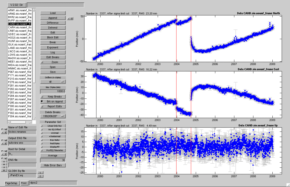
Below is an example of loading the CAND site after the ParkEX.eq file has been loaded (using the L button next to the GLOBK Eq file box). (The ParkEX.eq file is in directory above the time series and its name is given as ../ParkEX.eq). On this figure, the red line show log postseismic breaks (from the San Simeon and Parkfield earthquakes), the black line is a simple earthquake offset (due to Hector Mine). Blue vertical lines are exponential decay postseismic jumps. Green vertical lines would be offsets due to antenna, radome or receiver changes (none shown here). There have been some data edited in the eq file using the _XPS rename option.
Dir button
The box at top of the screen allows the specification of a directory where the time series files are located. The name is typed in text box and dir pressed to load the names of the sites in the directory.
Center column buttons:
Load:
This loads the data from the selected site. When mb_ files are used the data are in the output format from multibase. An example of an mb_file is shown below. There are three header lines on the file and second line is used to determine total value of the component being plotted. The entries in the time series are the <10-meter part of the component being plotted. The format of the file name (i.e., mb_ABCD_XYZ.datN where ABCD_XYZ is the site name, and the N at the end of the name is used to denoted component with 1 being North, 2 being East and 3 being height.
Globk Analysis
AZU1_GHT to N Solution
1 + 3798890.892 m
1999.7931
0.8572 0.0017
…
2002.7767
0.9247 0.0020
2002.7795
0.9241 0.0020
Alternatively PBO format may be used where all components
appear in one file. An example is
shown below:
% more CAND.sio.noamf_frame.pos
PBO Station Position Time Series. Reference Frame : ITRF2005
Format Version: 1.0.2
4-character ID: CAND
Station name :
CAND_sio.noamf
First Epoch
: 19990821 120000
Last Epoch
: 20090110 120000
Release Data :
20090127 142905
XYZ Reference position :
-2619024.97105 -4458011.11937
3723079.05281 (ITRF2005)
NEU Reference position : 35.9393527545 239.5663046682
568.39395 (ITRF2005/WGS84)
19990821 120000
51411.5000 -2619024.95323 -4458011.15090
3723079.01190 0.00399 0.00566 0.00453
0.000 0.000 0.000 35.9393523600 239.5663050154 568.38464 -0.04392 0.03129
-0.00931
0.00228 0.00228 0.00768 0.000
0.000 0.000 noamf
19990822 120000
51412.5000 -2619024.95520 -4458011.15382
3723079.01489 0.00341 0.00517 0.00433
0.000 0.000 0.000 35.9393523632 239.5663050130 568.38924 -0.04356 0.03108
-0.00471
0.00205 0.00205 0.00696 0.000
0.000 0.000 noamf
….
20090109 120000 54840.5000 -2619024.97437 -4458011.09518 3723079.07615 0.00404 0.00644 0.00532 0.000
0.000 0.000 35.9393530262 239.5663045007 568.39212 0.03025 -0.01510
-0.00182
0.00257 0.00257 0.00845 0.000
0.000 0.000 noamf
20090110 120000
54841.5000 -2619024.97806 -4458011.09468
3723079.07064 0.00298 0.00480 0.00387
0.000 0.000 0.000 35.9393529784 239.5663044626 568.39005 0.02493 -0.01853
-0.00390
0.00185 0.00185 0.00626 0.000
0.000 0.000 noamf
Append:
Appends another site's data onto previously loaded data. This option may be used multiple times to append several site names. Most often append is used to re-connect sites that have different names due to earthquakes and renames in GLOBK. Other buttons on the screen determine the precise operations during appends. By default, Break on Append (Brk on Append button) is set which means that a break is automatically added at the end of the last data set loaded or appended. For this feature to work correctly, data must be loaded and appended in time order. Since the symbols used to plot the data change with each append, the breaks in data can be found by looking at the symbols. The other option on append is to check the O box next to the append button which will calculate and remove an offset between the original and appended data based on overlapping data times. Statistics of the overlap are written to the Matlab Window. Normally Break on Append would be turned off during this operation.
All data is displayed during the load and append steps.
Detrend:
Removes a linear rate and offsets at breaks plus any parameters set in the Parameter Set box (see below). During the detrend operation, the conditions on the maximum sigma of the coordinate estimates (Max Sigma box) will be applied, and the detrend will be iterated to remove outlier data based on the Max Outlier box. The default all setting will not apply a n-sigma edit. Levels of 5/4/3/2 and 1-sigma outlier removal can be set. (Small values of this condition can lead to all data being deleted). The sigma used in the condition is scaled by the NRMS fit to the linear trend. The results of the parameter estimates are written to the Matlab window and appear in a figure in the top-right hand corner of the computer screen. One sigma error estimates for the model fit are shown as thin red lines on the plot after detrending.
Edit:
Edit allows individual points to be deleted from the time series. Using right-click keeps tsview in edit mode to allow multiple points to be edited.
Block Edit:
Allows areas to be selected for editing using a click and drag technique. Block edit must be re-selected to allow multiple blocks to be edited.
Break:
Allows times for breaks to be graphically selected. The List of breaks currently active appears in the Delete Break popup menu. A simple offset break is displayed with a green vertical line
Exponential:
Allows specification of an exponential fit to a break at the time of an earthquake. The selection mode is to click at the start of the exponential and to drag to the 1/e point. The final selection can be edited with the edit break button below. The estimated offset is the co-seismic offset. The exponential term is the accumulated post-seismic motion. An exponential break is displayed with a blue vertical line and a thick horizontal line showing the 1/e time.
The expression used is:
![]()
where C is co-seismic offset, epsilon is the amplitude
of the exponential term, tau is the decay time and ![]() is a Heavy-side step function at the time of the
earthquake (teq). If
the Exp/Ln rates option is set, separate
velocities before and after the earthquake are estimated.
is a Heavy-side step function at the time of the
earthquake (teq). If
the Exp/Ln rates option is set, separate
velocities before and after the earthquake are estimated.
Logarithmic:
Allows specification of a logarithmic function to be fit after an Earthquake. Similar to the exponent file except the click and drag selects the start of the data to be used in the logarithmic fit and time normalization of the logarithm fit (allows the curvature of the logarithm function to be controlled. Normally the drag direction is to the left. The start of the bar at the bottom shows the start time of the logarithmic function. A logarithmic break is displayed with a vertical red line and a thick horizontal line show the time constant to the logarithm function. The logarithm fit uses a natural logarithm (LN) with years as the time argument,
![]()
where C is the co-seismic offset, lamda is the amplitude of the logarithmic term, tau is the time constant of the logarithmic function.
Edit Breaks:
Displays a dialog box that allows the break characteristics to be edited. (Breaks are deleted using the Delete Break button explained below). The type of break can be changed with this option. The break types are: BR Standard simple offset at time of break; EX Exponent fit characterized by the start date and the 1/e time of the exponent fit; LN Logarithmic fit characterized by the date of the earthquake and the time constant tau. All times are given as year month day hour min. Time constants are in days.
Zoom:
Standard Matlab zoom feature that allows areas of individual components of the time series to be viewed. Double clicking should un-zoom the view.
Span:
Allows a span of time to shown (click and drag box). All components of the original are re-displayed. In this view, the time series is not detrended.
Save:
Save operates with the boxes below the station names. Three types of outputs can be saved depending on whether the W buttons (write) are set next the file names (by default all three file types will be written). The Edit file generates a set of renames for GLOBK. This file may be used with the eq_file command in the GLOBK command file. The ensum output files is the same format as generated by the ENSUM program. An example of the individual station files is ts_CAND.sio.noamf_frame.det
Max Outlier (n-sigma):
An automatic outlier rejection criterion used in an iterative de-trending
Max Sigma (mm):
Removes points with large error bars during de-trending.
Keep Breaks:
When checked, the breaks from previous loads are retained when new sites are loaded.
Brk on Append:
Adds a break at the end of the previous data set when a new site is appended.
Report Edits:
Prints details of the editing to the Matlab window.
Delete Breaks:
This is a popup menu that shows the dates of the breaks being used. Breaks which appear with an * after the data are either exponent or logarithm fits (see Edit Break). If one of these is selected, then it will be removed. If the mouse is clicked outside the area of the list then no breaks will be deleted.
Parameter Set:
In addition to linear trends and offsets, annual and semiannual signals can be estimated.
Linear Only Resid
When this button is checked, the estimated annual and semiannual, exponent and logarithm coefficients are not removed from the data (the offset values associated with these breaks are removed). A plot of these signals is superimposed on the residual plot.
No EQ offset
When this button is checked, the estimated offsets at times
of earthquakes are not removed from the plot when linear only residuals are
displayed (Breaks if BR type are removed).
+Annual
estimates an annual signal (cos and sin based on Jan 1).
+Semiannual
estimates a semiannual signal (cos and sin based on Jan 1).
Exp/Ln Rates
Estimates a new rate after an exponential or logarithm break. The output parameter is the difference in rate between the pre- and post-break data.
RealSigma
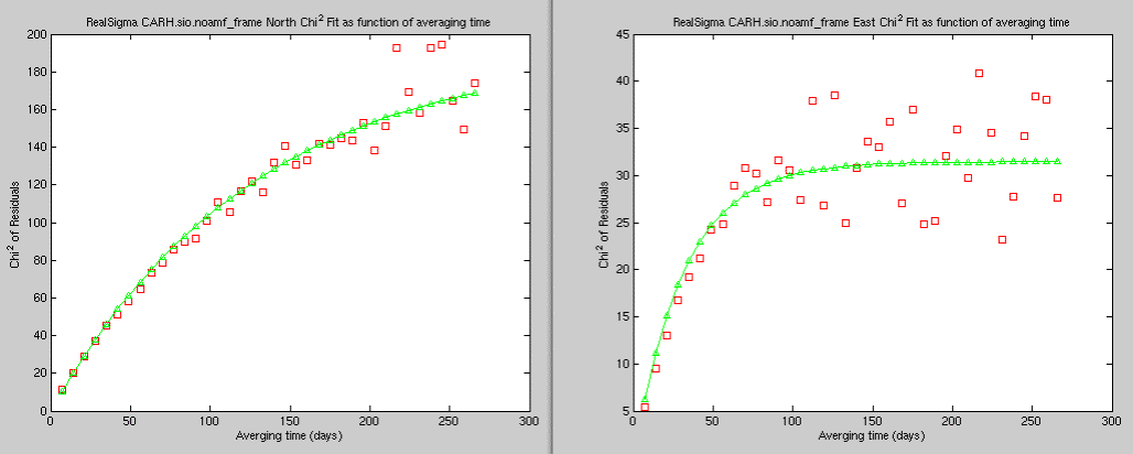
"Realistic Sigma" calculation. The algorithm used here assumes that the noise process is a first order Gauss Markov process. The time series residuals to the fit to the data are averaged over increasingly longer intervals, and the chi^2-per-degree of freedom of the averaged values are computed. For nearly all times series, the chi^2-per-degree of freedom (chi^2/f) increases with increasing averaging time. (For a white noise process, the value would remain constant.) The rate of increase of chi^2/f is used to fit a correlation time for the process noise, and this correlation time is used to compute realistic sigmas for the fits by scaling the white-noise estimates of the sigmas. The chi^2/f values can be viewed with the DisplayFit option below.
DisplayFit
Used with the RealSigma option and shows the changes in chi^2/f with increasing averaging time, and the fit of the correlated noise model to the computed values.
Post EQ time series
Checking this box will output weekly values up to 2010 of
the log or exponential contributions to postseismic deformation. File names start with PVO and are
overwritten each time the detrend button is pressed (while the Post EQ time
series box is checked). Separate
files for N, E and U are written.
The start time is the first log or exponential break and all subsequent
log and exponential breaks are added. The accumulated offset and the derivative
of the offset along with the standard deviations are given along with the
correlation between the offset and rate.
WARNING: The option does not work if Exp/Ln Rates (ie., differerent
linear rates are after earthquakes) has been selected.
Average
Averages the residuals of the time series over the interval in days given in the box. An optional year month day hour min (truncated to desired level) may be given to specify a boundary for the averaging. This feature is useful when averaging around the time of an earthquake. The error bars on the original time series are removed and the scales on the figures changed to match the size of the averaged residuals. The bold text at the tops of each figure, give the statistics of the averaged residuals. This feature may be used at anytime including when time series are first loaded.
Hide Error Bars
Removes the error bars from time series plots.
Input ENS file:
Allows a summary file from ENSUM or tsfit to be read in and the sites sorted according to the buttons on the left of the Input ENS file boxes. When the H button is clicked, the summary file is read and the site names sorted by horizontal RMS scatter (largest values at the top of the list). If the N box is checked, the NRMS is used for sorting, otherwise the WRMS is used. When the V button is clicked, the same operations occur except the vertical RMS values are used. The W button uses the worst of the horizontal and vertical RMS scatters. The A button returns the site list an alphabetical list.
GLOBK EQ File
A globk earthquake file containing earthquakes, breaks, and
data editing (renames to _XPS or _XCL) may be given. Clicking the L button loads the file and Clicking C once
will clear all the earthquake and rename entries. Clicking C a second time will remove the file name from the
EQ file box.
Print and Page Setup:
These buttons allow the page setup (paper orientation, fitting of the figure on the page) to be set. The print button prints the figure using the arguments given in the box next to it. Some typical options are:
-d<device> with device being psc for color post script; png for portable network graphics; jpeg of jpeg image
-r<NN> sets resolution for image formats. NN is dots per inch with 72 being appropriate from screen resolution.
-P<queue> to set the printer queue to be used
<filename> the last argument can be a file name to which the print is sent.
Example: -dpng –r72 –noui Test.png outputs figures to portable network graphics (PNG) file.
The -noui option must be used and this stops the GUI information from being printed. When run under Matlab, the functionality of these boxes is available under the file menu.
Example screen view and output
Example 1: Annual and logarithmic fit to data and averaging, and use of "linear only" residuals
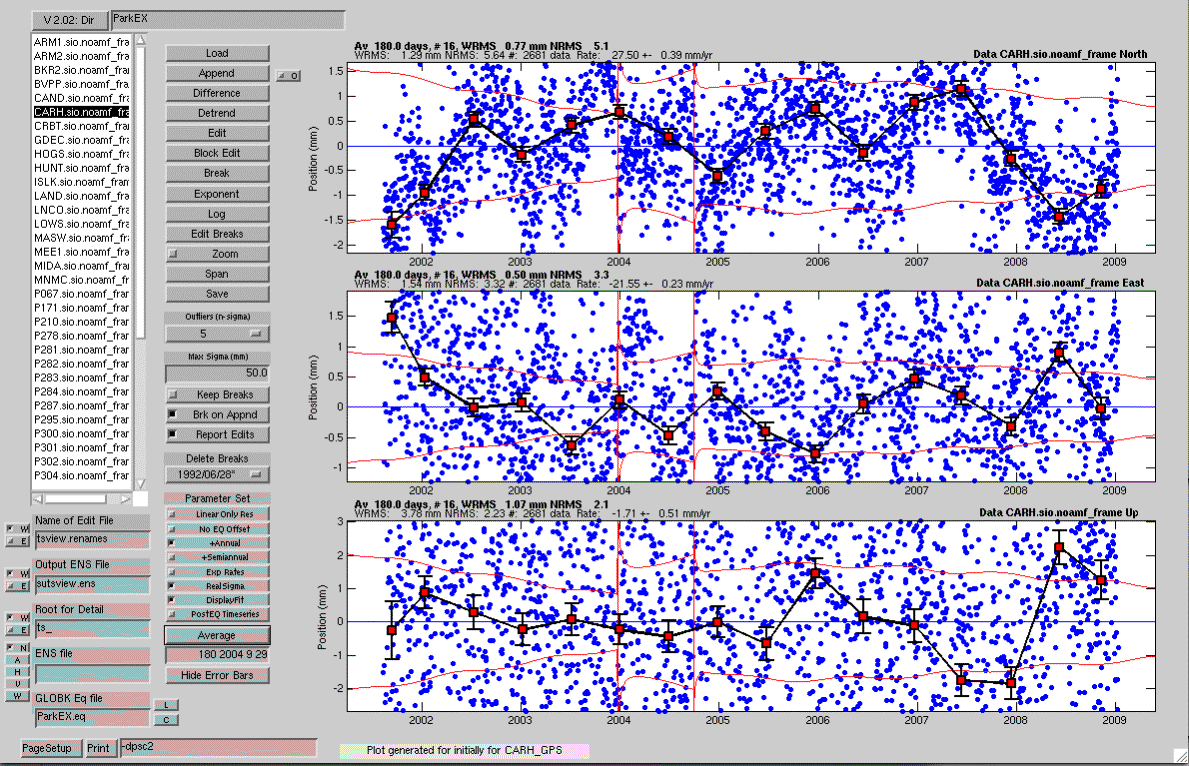
Below is an example of a de-trended time series with annual terms estimated, and logarithmic fits after the San Simeon and Parkfield earthquakes (these were read in from the globk EQ file but could have been entered with the Edit Break button). A 4-sigma editing condition was used and with the Report Edits feature on, the details of the deleted data are printed to the Matlab command window or terminal screen. The realistic sigma option was also used with the Display fit option selected. The default sigma limit was reduced to 50 mm to remove 3 points with large error bars. The output below comes to the screen and shows the data points edited due to the N-sigma condition, correlation information from the "Realistic Sigma" option, statistics of the fit and the estimated parameters. In this case, there are possible offsets from Landers and Hector Mine earthquakes (no log or exponential postseismic estimates for this example case) but since there are no data, the estimates are zero.
----------------------------------------------
Edit 1137
Date 2004 9 29 12 0 Res 10.0 +- 1.8 North
Edit 1834
Date 2006 8 28 12 0 Res -20.2 +-
3.4 North
Edit 1137
Date 2004 9 30 12 0 Res 6.0 +- 1.7 North
Computing Realistic Sigmas
RealSigma white dchi 0.405384
NRMS Realistic 5.63; Correlation time 128.00 days
Detrend of CARH.sio.noamf_frame North
WRMS:
1.29 mm NRMS: 5.63 #: 2683 data
Mean
-24.15 +- 303.00 mm
Rate 27.50
+- 0.39 mm/yr
Annual Cos
0.56 +- 0.32 mm
Annual Sin
-0.64 +- 0.31 mm
EQBrk 1992 6 28
12 0
0.00 +- 214.25 mm
EQBrk 1999 10 16 9
46
-0.00 +- 214.25 mm
OffLn 2003 12 22 19 15 dOf 1.0 -3.22 +- 3.15 mm
Log 2003 12
22 19 15 dOf 1.0
-0.85 +- 0.70 mm
OffLn 2004 9 28 17
15 dOf 1.0
-27.80 +- 2.59 mm
Log
2004 9 28 17 15 dOf
1.0 12.58
+- 0.54 mm
Edit
78 Date 2001 10 29 12 0
Res 8.0 +- 1.9 East
Edit 1834
Date 2006 8 31 12 0 Res -26.7 +-
3.5 East
Computing Realistic Sigmas
RealSigma white dchi 0.604784
NRMS Realistic 3.32; Correlation time 32.00 days
Detrend of CARH.sio.noamf_frame East
WRMS:
1.54 mm NRMS: 3.32 #: 2681 data
Mean
35.97 +- 178.42 mm
Rate
-21.55 +- 0.23 mm/yr
Annual Cos
0.66 +- 0.19 mm
Annual Sin
0.01 +- 0.18 mm
EQBrk 1992 6 28
12 0
0.00 +- 126.16 mm
EQBrk 1999 10 16 9
46
0.00 +- 126.16 mm
OffLn 2003 12 22 19 15 dOf 1.0 -9.38 +- 1.85 mm
Log 2003 12
22 19 15 dOf 1.0
-0.95 +- 0.41 mm
OffLn 2004 9 28 17
15 dOf 1.0
26.05 +- 1.52 mm
Log
2004 9 28 17 15 dOf
1.0 -11.02
+- 0.32 mm
Computing Realistic Sigmas
RealSigma white dchi 0.424070
NRMS Realistic 2.23; Correlation time 32.00 days
Detrend of CARH.sio.noamf_frame Up
WRMS:
3.78 mm NRMS: 2.23 #: 2681 data
Mean
-4.02 +- 394.43 mm
Rate
-1.71 +- 0.51 mm/yr
Annual Cos
-1.53 +- 0.42 mm
Annual Sin
3.27 +- 0.41 mm
EQBrk 1992 6 28
12 0
0.00 +- 278.90 mm
EQBrk 1999 10 16 9
46
0.00 +- 278.90 mm
OffLn 2003 12 22 19 15 dOf 1.0 -1.12 +- 4.12 mm
Log 2003 12
22 19 15 dOf 1.0
-0.27 +- 0.91 mm
OffLn 2004 9 28 17
15 dOf 1.0
-3.03 +- 3.37 mm
Log
2004 9 28 17 15 dOf
1.0
2.16 +- 0.70 mm
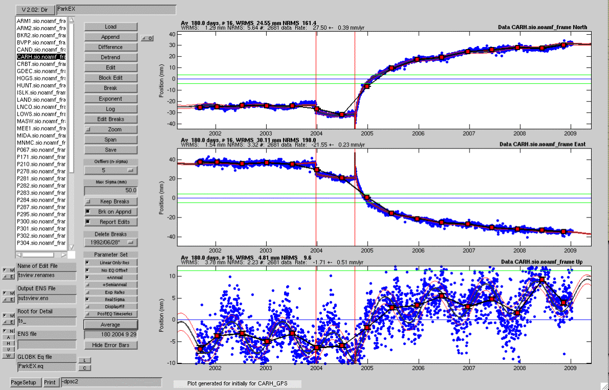
The figure below shows residuals to the fit with just the linear velocity removed (any standard breaks due to antenna and other changes would also be removed here). The No EQ offset option is set so the co-seismic offsets have not been removed. The residuals have been averaged over 180-day periods and the boundary of the averaging windows has been set to coincide with the Parkfield earthquake. The grey line (seen easiest in the Up plot) is the model itself and the redlines in either side are +- 1 sigma estimates of the noise in the model.
The figure below show the output from the Display Fit option for the N and E components when realistic sigmas are estimated (there is also a plot for Up but it is not shown). The red squares are the estimated chi^2/f for the residuals as a function of averaging time and the green triangles are the first-order Gauss-Markov model fits to the averaging dependence. The white noise estimated sigmas are multiplied by the value of the green curve at infinite averaging time corrected for the error bar scaling. (The later is based on the chi^2/f of the differences between adjacent data points.)
The figure below shows the residuals when all of the model terms are removed. Again 180-day averaged residuals are also shown.
